(Warning: These materials may be subject to lots of typos and errors. We are grateful if you could spot errors and leave suggestions in the comments, or contact the author at yjhan@stanford.edu.)
In this lecture, we establish the asymptotic lower bounds for general statistical decision problems. Specifically, we show that models satisfying the benign local asymptotic normality (LAN) condition are asymptotically equivalent to a Gaussian location model, under which the Hájek–Le Cam local asymptotic minimax (LAM) lower bound holds. We also apply this theorem to both parametric and nonparametric problems.
1. History of Asymptotic Statistics
To begin with, we first recall the notions of the score function and Fisher information, which can be found in most textbooks.
Definition 1 (Fisher Information) A family of distributions
on
is quadratic mean differentiable (QMD) at
if there exists a score function
such that
In this case, the matrix
exists and is called the Fisher information at
.

R. A. Fisher popularized the above Fisher information and the usage of the maximum likelihood estimator (MLE) starting from 1920s. He believes that, the Fisher information of a statistical model characterizes the fundamental limits of estimating 

- For any asymptotically normal estimators
such that
for any
, there must be
- The MLE satisfies that
for any
.

Although the second conjecture is easier to establish assuming certain regularity conditions, the first conjecture, which seems to be correct by the well-known Cramér-Rao bound, actually caused some trouble when people tried to prove it. The following example shows that (1) may be quite problematic.
Example 1 Here is a counterexample to (1) proposed by Hodges in 1951. Let
, and consider a Gaussian location model where
are i.i.d. distributed as
. A natural estimator of
, and the Fisher information is
. The Hodges’ estimator is constructed as follows:
It is easy to show that
, with
for non-zero
for
. Consequently, (1) does not hold for the Hodges’ estimator. The same result holds if the threshold
in (2) is changed by any sequence
with
and
.

Hodges’ example suggests that (1) should at least be weakened in appropriate ways. Observing the structure of Hodges’ estimator (2) carefully, there can be three possible attempts:
- The estimator
- Although the Hodges’ estimator satisfies the asymptotic normal condition, i.e.,
weakly converges to a normal distribution under
, for any non-zero perturbation
, the sequence
does not weakly converge to the same distribution under
. Hence, we may expect that (1) actually holds for more regular estimator sequences.
- Let
be the risk function of the estimator
, while
for
. In other words, the worst-case risk over an interval of size
around
, which is considerably larger than the single point
It turns out that all these attempts can be successful, and the following theorem summarizes the key results of asymptotic statistics developed by J. Hájek and L. Le Cam in 1970s.
Theorem 2 (Asymptotic Theorems) Let
at
. Let
be differentiable at
, and
be an estimator sequence of
.
1. (Almost everywhere convolution theorem) If
converges in distribution to some probability measure
for every
is non-singular for every
such that
for Lebesgue almost everydenotes the convolution.
2. (Convolution theorem) If
, and
weakly converges to the same limit under
, then there exists some probability measure
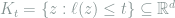
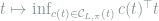
3. (Local asymptotic minimax theorem) Let
be a bowl-shaped loss function, i.e.,
and the sublevel sets
are convex for all
. Then
with.


We will be primarily interested in the local asymptotic minimax (LAM) theorem, for it directly gives general lower bounds for statistical estimation. This theorem will be proved in the next two sections using asymptotic equivalence between models, and some applications will be given in the subsequent section.
2. Gaussian Location Model
In this section we study the possibly simplest statistical model, i.e., the Gaussian location model, and will show in the next section that all regular models will converge to it asymptotically. In the Gaussian location model, we have 


Theorem 3 For any bowl-shaped loss
for

The proof of Theorem 3 relies on the following important lemma for Gaussian random variables.
Lemma 4 (Anderson’s Lemma) Let

Proof: For 


it suffices to show that 

Theorem 5 (Prépoka-Leindler Inequality, or Functional Brunn-Minkowski Inequality) Let
and
be non-negative real-valued measurable functions on
, with
Then


Let 


and 


Finally, by symmetry of 

Now we are ready to prove Theorem 3.
Proof: Consider a Gaussian prior 


Since this inequality holds for any 


3. Local Asymptotic Minimax Theorem
In this section, we show that regular statistical models converge to a Gaussian location model asymptotically. To prove so, we shall need verifiable criterions to establish the convergence of Le Cam’s distance, as well as the specific regularity conditions.
3.1. Likelihood Ratio Criteria for Asymptotic Equivalence
In Lecture 3 we introduced the notion of Le Cam’s model distance, and showed that it can be upper bounded via the randomization criterion. However, designing a suitable transition kernel between models is too ad-hoc and sometimes challenging, and it will be helpful if simple criteria suffice.
The main result of this subsection is the following likelihood ratio criteria:
Theorem 6 Let
and
be finite statistical models. Further assume that
is homogeneous in the sense that any pair in
is mutually absolutely continuous. Define
as the likelihood ratios, and similarly for
. Then
if the distribution of
under
weakly converges to that of
under
.
![L_{n,i}(x_n) = \frac{dP_{n,i}}{dP_{n,0}}(x_n), \qquad i\in [m]](https://s0.wp.com/latex.php?latex=+L_%7Bn%2Ci%7D%28x_n%29+%3D+%5Cfrac%7BdP_%7Bn%2Ci%7D%7D%7BdP_%7Bn%2C0%7D%7D%28x_n%29%2C+%5Cqquad+i%5Cin+%5Bm%5D+&bg=ffffff&fg=7f8d8c&s=0&c=20201002)
In other words, Theorem 6 states that a sufficient condition for asymptotic equivalence of models is the weak convergence of likelihood ratios. Although we shall not use that, this is also a necessary condition. The finiteness assumption is mainly for technical purposes, and the general case requires proper limiting arguments.
To prove Theorem 6, we need the following notion of standard models.
Definition 7 (Standard Model) Let
, and
be its Borel
-algebra. A standard distribution
on
is a probability measure such that
for any
. The model
is called the standard model of

The following lemma shows that any finite statistical model can be transformed into an equivalent standard form.
Lemma 8 Let
be a standard model with standard distribution
under mean measure
. Then
.
Proof: Since ![\mathop{\mathbb E}_{\mu}[t_i] = \mathop{\mathbb E}_{\overline{P}}[dP_i/d\overline{P}]=1](https://s0.wp.com/latex.php?latex=%5Cmathop%7B%5Cmathbb+E%7D_%7B%5Cmu%7D%5Bt_i%5D+%3D+%5Cmathop%7B%5Cmathbb+E%7D_%7B%5Coverline%7BP%7D%7D%5BdP_i%2Fd%5Coverline%7BP%7D%5D%3D1&bg=ffffff&fg=7f8d8c&s=0&c=20201002)


![\mathop{\mathbb E}_{Q_i}[h(t)] = \mathop{\mathbb E}_{\overline{P}}\left[h(t)\frac{dP_i}{d\overline{P}} \right] = \mathop{\mathbb E}_{\mu}\left[h(t) t_i \right]](https://s0.wp.com/latex.php?latex=+%5Cmathop%7B%5Cmathbb+E%7D_%7BQ_i%7D%5Bh%28t%29%5D+%3D+%5Cmathop%7B%5Cmathbb+E%7D_%7B%5Coverline%7BP%7D%7D%5Cleft%5Bh%28t%29%5Cfrac%7BdP_i%7D%7Bd%5Coverline%7BP%7D%7D+%5Cright%5D+%3D+%5Cmathop%7B%5Cmathbb+E%7D_%7B%5Cmu%7D%5Cleft%5Bh%28t%29+t_i+%5Cright%5D+&bg=ffffff&fg=7f8d8c&s=0&c=20201002)
for any measurable function 


Lemma 8 helps to convert the sample space of all finite models to the simplex 
Lemma 9 Let
and
be two finite models with standard distributions
respectively. Then
where
denotes the Dudley’s metric between probability measures
, and the supremum is taken over all measurable functions
with
and
for any
.

Remark 1 Recall that Dudley’s metric metrizes the weak convergence of probability measures on a metric space with its Borel
Proof: Similar to the proof of the randomization criterion (Theorem 5 in Lecture 3), the following upper bound on the model distance holds:

where 


where the set 

Since the diameter of 


Finally we are ready to present the proof of Theorem 6. Note that there is a bijective map between 

Remark 2 The continuous mapping theorem for weak convergence states that, if Borel-measurable random variables
converges weakly to
on a metric space, and
is a function continuous on a set
such that
, then
also converges weakly to
. Note that the function
3.2. Locally Asymptotically Normal (LAN) Models
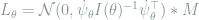
Motivated by Theorem 6, in order to prove that certain models asymptotically become normal, we may show that the likelihood functions weakly converge to those in the normal model. Note that for the Gaussian location model 

where 

Definition 10 (Local Asymptotic Normality) A sequence of models
with
is called locally asymptotically normal (LAN) with central sequence
and Fisher information matrix
if
with
under
, and
converges to zero in probability under

Based on the form of the likelihood ratio in (4), the following theorem is then immediate.
Theorem 11 If a sequence of models
satisfies the LAN condition with Fisher information matrix
for
.
Proof: Note that for any finite sub-model, Slutsky’s theorem applied to (4) gives the desired convergence in distribution, and clearly the Gaussian location model is homogeneous. Now applying Theorem 6 gives the desired convergence. We leave the discussion of the general case in the bibliographic notes.
Now the only remaining task is to check the likelihood ratios for some common models and show that the LAN condition is satisfied. For example, for QMD models 

where intuitively by CLT and LLN will arrive at the desired form (4). The next proposition makes this intuition precise.
Proposition 12 Let
with Fisher information matrix
, with
satisfies the LAN condition with Fisher information
Proof: Write 

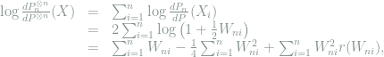
where 


Moreover, 
![\mathop{\mathbb E}\left[\sum_{i=1}^n W_{ni}\right] = -n\int (\sqrt{dP_n} - \sqrt{dP})^2 \rightarrow - \frac{1}{4}\mathop{\mathbb E}_P[g(X)^2].](https://s0.wp.com/latex.php?latex=+%5Cmathop%7B%5Cmathbb+E%7D%5Cleft%5B%5Csum_%7Bi%3D1%7D%5En+W_%7Bni%7D%5Cright%5D+%3D+-n%5Cint+%28%5Csqrt%7BdP_n%7D+-+%5Csqrt%7BdP%7D%29%5E2+%5Crightarrow+-+%5Cfrac%7B1%7D%7B4%7D%5Cmathop%7B%5Cmathbb+E%7D_P%5Bg%28X%29%5E2%5D.+&bg=ffffff&fg=7f8d8c&s=0&c=20201002)
Consequently, we conclude that
![\sum_{i=1}^n W_{ni} = \frac{1}{\sqrt{n}}\sum_{i=1}^n g(X_i) -\frac{1}{4}\mathop{\mathbb E}_P[g(X)^2] + o_P(1).](https://s0.wp.com/latex.php?latex=+%5Csum_%7Bi%3D1%7D%5En+W_%7Bni%7D+%3D+%5Cfrac%7B1%7D%7B%5Csqrt%7Bn%7D%7D%5Csum_%7Bi%3D1%7D%5En+g%28X_i%29+-%5Cfrac%7B1%7D%7B4%7D%5Cmathop%7B%5Cmathbb+E%7D_P%5Bg%28X%29%5E2%5D+%2B+o_P%281%29.+&bg=ffffff&fg=7f8d8c&s=0&c=20201002)
For the second term, the QMD condition gives 
![\sum_{i=1}^n W_{ni}^2 = \mathop{\mathbb E}_P[g(X)^2] + o_P(1)](https://s0.wp.com/latex.php?latex=%5Csum_%7Bi%3D1%7D%5En+W_%7Bni%7D%5E2+%3D+%5Cmathop%7B%5Cmathbb+E%7D_P%5Bg%28X%29%5E2%5D+%2B+o_P%281%29&bg=ffffff&fg=7f8d8c&s=0&c=20201002)

![\max_{i\in [n]} | r(W_{ni}) | = o_P(1)](https://s0.wp.com/latex.php?latex=%5Cmax_%7Bi%5Cin+%5Bn%5D%7D+%7C+r%28W_%7Bni%7D%29+%7C+%3D+o_P%281%29&bg=ffffff&fg=7f8d8c&s=0&c=20201002)
In other words, Proposition 12 implies that all regular statistical models locally look like normal, where the local radius is 
3.3. Proof of LAM Theorem
Now we are ready to glue all necessary ingredients together. First, for product QMD statistical models, Proposition 12 implies that LAN condition is satisfied for the local model around any chosen parameter 

Theorem 13 (LAM, restated) Let
, and any bowl-shaped loss function
. Then
with
Note that here the compactness of the action space is required for the limiting arguments, while all our previous analysis consider finite models. Our arguments via model distance are also different from those used by H\'{a}jek and Le Cam, where they introduced the notion of contiguity to arrive at the same result with weaker conditions. Further details of these alternative approaches are referred to the bibliographic notes.
4. Applications and Limitations
In this section, we will apply the LAM theorem to prove asymptotic lower bounds for both parametric and nonparametric problems. We will also discuss the limitations of LAM to motivate the necessity of future lectures.
4.1. Parametric Entropy Estimation
Consider the discrete i.i.d. sampling model 


under the mean squared loss. We can apply LAM to prove a local minimax lower bound for this problem.
First we compute the Fisher information of the multinomial model 

By the matrix inversion formula 
Now choosing 

![\inf_{\hat{H}} \sup_{P\in \mathcal{M}_k} \mathop{\mathbb E}_P (\hat{H} - H(P))^2 \ge \frac{1+o_n(1)}{n} \sup_{P\in \mathcal{M}_k} \text{Var}\left[\log\frac{1}{P(X)}\right].](https://s0.wp.com/latex.php?latex=+%5Cinf_%7B%5Chat%7BH%7D%7D+%5Csup_%7BP%5Cin+%5Cmathcal%7BM%7D_k%7D+%5Cmathop%7B%5Cmathbb+E%7D_P+%28%5Chat%7BH%7D+-+H%28P%29%29%5E2+%5Cge+%5Cfrac%7B1%2Bo_n%281%29%7D%7Bn%7D+%5Csup_%7BP%5Cin+%5Cmathcal%7BM%7D_k%7D+%5Ctext%7BVar%7D%5Cleft%5B%5Clog%5Cfrac%7B1%7D%7BP%28X%29%7D%5Cright%5D.+&bg=ffffff&fg=7f8d8c&s=0&c=20201002)
Note that 
4.2. Nonparametric Entropy Estimation
Consider a continuous i.i.d. sampling model from some density, i.e., 

As before, we would like to prove a local minimax lower bound for the mean squared error around any target density 
Let 


Setting 

and consequently

Since our choice of the test function 

Clearly, this value is attained for the test function 

Therefore, the parametric lower bound for nonparametric entropy estimation is

4.3. Limitations of Classical Asymptotics
The theorems from classical asymptotics can typically help to prove an error bound
- Non-asymptotic vs. asymptotic: Asymptotic bounds are useful only in scenarios where the problem size remains fixed and the sample size grows to infinity, and there is no general guarantee of when we have entered the asymptotic regime (it may even require that
). In practice, essentially all recent problems are high-dimensional ones where the number of parameters is comparable to or even larger than the sample size (e.g., an over-parametrized neural network), and some key properties of the problem may be entirely obscured in the asymptotic regime.
- Parametric vs. nonparametric: The results in classical asymptotics may not be helpful for a large quantity of nonparametric problems, where the main problem is the infinite-dimensional nature of nonparametric problems. Although sometimes the parametric reduction is helpful (e.g., the entropy example), the parametric rate
, the worst-case test function will actually give a vacuous lower bound (which is infinity).
- Global vs. local: As the name of LAM suggests, the minimax lower bound here holds locally. However, the global structure of some problems may also be important, and the global minimax lower bound may be much larger than the supremum of local bounds over all possible points. For example, in Shannon entropy estimation, the bias is actually dominating the problem and cannot be reflected in local methods.
To overcome these difficulties, we need to develop tools to establish non-asymptotic results for possibly high-dimensional or nonparametric problems, which is the focus of the rest of the lecture series.
5. Bibliographic Notes
The asymptotic theorems in Theorem 2 are first presented in Hájek (1970) and Hájek (1972), and we refer to Le Cam (1986), Le Cam and Yang (1990) and van der Vaart (2000) as excellent textbooks. Here the approach of using model distance to establish LAM is taken from Section 4, 6 of Liese and Miescke (2007); also see Le Cam (1972).
There is another line of approach to establish the asymptotic theorems. A key concept is the contiguity proposed by Le Cam (1960), which enables an asymptotic change of measure. Based on contiguity and LAN condition, the distribution of any (regular) estimator under the local alternative can be evaluated. Then the convolution theorem can be shown, which helps to establish LAM; details can be found in van der Vaart (2000). LAM theorem can also be established directly by computing the asymptotic Bayes risk under proper priors; see Section 6 of Le Cam and Yang (1990).
For parametric or nonparametric entropy estimation, we refer to recent papers (Jiao et al. (2015) and Wu and Yang (2016) for the discrete case, Berrett, Samworth and Yuan (2019) and Han et al. (2017) for the continuous case) and the references therein.
- Jaroslav Hájek, A characterization of limiting distributions of regular estimates. Zeitschrift für Wahrscheinlichkeitstheorie und verwandte Gebiete 14.4 (1970): 323-330.
- Jaroslav Hájek, Local asymptotic minimax and admissibility in estimation. Proceedings of the sixth Berkeley symposium on mathematical statistics and probability. Vol. 1. 1972.
- Lucien M. Le Cam, Asymptotic methods in statistical theory. Springer, New York, 1986.
- Lucien M. Le Cam and Grace Yang, Asymptotics in statistics. Springer, New York, 1990.
- Aad W. Van der Vaart, Asymptotic statistics. Vol. 3. Cambridge university press, 2000.
- Friedrich Liese and Klaus-J. Miescke. Statistical decision theory. Springer, New York, NY, 2007.
- Lucien M. Le Cam, Limits of experiments. Proceedings of the Sixth Berkeley Symposium on Mathematical Statistics and Probability, Volume 1: Theory of Statistics. The Regents of the University of California, 1972.
- Lucien M. Le Cam, Locally asymptotically normal families of distributions. University of California Publications in Statistics 3, 37-98 (1960).
- Jiantao Jiao, Kartik Venkat, Yanjun Han, and Tsachy Weissman, Minimax estimation of functionals of discrete distributions. IEEE Transactions on Information Theory 61.5 (2015): 2835-2885.
- Yihong Wu and Pengkun Yang, Minimax rates of entropy estimation on large alphabets via best polynomial approximation. IEEE Transactions on Information Theory 62.6 (2016): 3702-3720.
- Thomas B. Berrett, Richard J. Samworth, and Ming Yuan, Efficient multivariate entropy estimation via
- Yanjun Han, Jiantao Jiao, Tsachy Weissman, and Yihong Wu, Optimal rates of entropy estimation over Lipschitz balls. arXiv preprint arXiv:1711.02141 (2017).