Lecture 6: Generalized Two-Point Method: Point vs. Mixture

(Warning: These materials may be subject to lots of typos and errors. We are grateful if you could spot errors and leave suggestions in the comments, or contact the author at yjhan@stanford.edu.)

In the last lecture we introduced Le Cam’s two-point method to establish information-theoretic lower bounds, where the target is to find two single hypotheses which are well separated while indistinguishable. However, restricting to two single hypotheses gives the learner a lot of information in many scenarios, and any pair of single hypotheses which are far apart becomes distinguishable. From another point of view, if we would like to mimic the Bayesian idea of using the least favorable prior, it is very unlikely that the least favorable prior is supported on only two points. Hence, in this lecture we generalize the two-point idea to the case where one point is a mixture of distributions, which suits well in various examples.

1. General Tools

1.1. A Motivating Example

We first discuss an example where the simple two-point method fails. Consider the following hidden clique detection problem: there is an underlying undirected simple graph $G$ with vertex set $[n]$ which either comes from an Erdös-Rényi graph $\mathcal{G}(n,1/2)$ (where each edge appears with probability $1/2$ independently), or there is a clique on $k$ vertices of $G$ and all other edges appear with probability $1/2$ independently. Recall that a clique is a complete graph where each two vertices are connected via an edge. The target is to reliably distinguish between these two cases, i.e., a vanilla Erdös-Rényi graph versus that planted with a hidden clique of size $k$ .

This task is a composite hypothesis testing problem, where $H_0$ consists of a single hypothesis where $G=\mathcal{G}(n,1/2)$ , while $H_1$ consists of a family of hypotheses depending on the precise location of the hidden clique. Of course, an Erdös-Rényi graph is unlikely to have large cliques, thus this task becomes easier when $k$ is large. Let $k_n>0$ be the threshold that the total error probability of the optimal test is at most $1/3$ when $k\ge k_n$ and is at least $1/3$ when $k<k_n$ .

We first try to use Le Cam’s two-point method to find a lower bound on $k_n$ . Let $P\in H_0$ be the distribution of $\mathcal{G}(n,1/2)$ , and $Q_S\in H_1$ be the distribution of the graph where there is a planted clique on the vertex set $S\subseteq [n]$ with $|S|=k$ . To compute the total variation distance between $P$ and $Q_S$ , note that with probability $2^{-\binom{k}{2}}$ the Erdös-Rényi graph has a clique supported on $S$ . Hence,

$\|P - Q_S \|_{\text{TV}} = 1 - 2^{-\binom{k}{2}}$

holds for any $S$ . As a result, we have $k=\Omega(1)$ to ensure that $\|P - Q_S \|_{\text{TV}}\ge 2/3$ , which is not an informative bound.

The problem with the above two-point approach is that, if the learner is told the exact location of the clique, she can simply look at the subgraph supported on that location and tell whether a clique is present. In other words, any single hypothesis from $H_1$ gives too much information to the learner. To overcome this difficulty, a natural idea is to take the support $S$ of the clique uniformly distributed on all size- $k$ subsets of $[n]$ , which is expected to result in a graph looking more similar to the Erdös-Rényi graph. This is exactly the central topic of this lecture.

1.2. Generalized Le Cam’s Method: Point vs. Mixture

As is shown in the previous example, there is need to generalize the Le Cam’s two-point method to the scenario where one of the points is a mixture of distributions. The theoretical foundation of the generalization is in fact quite simple, and the proof of the next theorem parallels that of Theorem 7 in Lecture 5.

Theorem 1 (Point vs. Mixture) Let $L: \Theta \times \mathcal{A} \rightarrow {\mathbb R}_+$ be any loss function, and there exist $\theta_0\in \Theta$ and $\Theta_1 \subseteq \Theta$ such that
$L(\theta_0, a) + L(\theta_1, a) \ge \Delta, \qquad \forall a\in \mathcal{A}, \theta_1\in \Theta_1,$
then for any probability measure $\mu$ supported on $\Theta_1$ , we have
$\inf_{\hat{\theta}} \sup_{\theta\in\Theta} \mathop{\mathbb E}_\theta L(\theta,\hat{\theta})\ge \frac{\Delta}{2}\cdot \left(1 - \|P_{\theta_0} - \mathop{\mathbb E}_{\mu(d\theta)}P_{\theta} \|_{\text{\rm TV}}\right).$

The main difficulties in the practical application of Theorem 1 lie in two aspects. First, it may be non-trivial to find the proper mixture $\mu$ and the support $\Theta_1$ . Second, upper bounding the total variation distance $\|P_{\theta_0} - \mathop{\mathbb E}_{\mu(d\theta)}P_{\theta} \|_{\text{\rm TV}}$ may be hard, especially when $P_\theta$ takes the form of $Q_\theta^{\otimes n}$ . The next section proposes a general tool to overcome the second difficulty, where we use various examples to illustrate the art of the first difficulty.

1.3. Upper Bounding the Divergence

To upper bound the divergence between a single distribution and a mixture of distributions, the next lemma shows that the $\chi^2$ -divergence is a proper choice.

Lemma 2 Let $(P_\theta)_{\theta\in\Theta}$ be a family of probability distributions parametrized by $\theta$ , and $Q$ be any fixed probability distribution. Then for any probability measure $\mu$ supported on $\Theta$ , we have
$\chi^2\left(\mathop{\mathbb E}_\mu [P_\theta], Q \right) = \mathop{\mathbb E}\left[ \int \frac{dP_\theta dP_{\theta'}}{dQ} \right] - 1,$
where the expectation is taken with respect to independent $\theta,\theta'\sim \mu$ .

Proof: Follows from the definition $\chi^2(P,Q) = \int\frac{(dP)^2}{dQ}-1$ and simple algebra. $\Box$

The advantages of Lemma 2 are two-fold. First, it factorizes well for tensor products:

$\chi^2\left(\mathop{\mathbb E}_\mu [P_\theta^{\otimes n}], Q^{\otimes n} \right) =\mathop{\mathbb E}\left[ \left( \int \frac{dP_\theta dP_{\theta'}}{dQ}\right)^n \right] - 1.$

This identity makes it more convenient to use $\chi^2$ -divergence to deal with the point-mixture scenario. Second, for many statistical models (and a proper choice of $Q$ ), the quantity

$\int \frac{dP_\theta dP_{\theta'}}{dQ}$

admits a simple closed-form expression in $(\theta,\theta')$ . We will see several examples in the rest of this lecture.

2. Examples of Testing Problems

In this section, we provide examples of composite hypothesis testing problems where the null hypothesis $H_0$ consists of a single probability distribution, while the alternative $H_1$ consists of a family of distributions. We will see that choosing a proper mixture and applying the tools in Lemma 2 gives desired lower bounds.

2.1. Hidden Clique Detection

Recall the hidden clique detection problem described in Section 1.1, where we aim to obtain tight lower bounds for the threshold $k_n$ on the clique size. As discussed, the point is chosen to be the single distribution $P$ for the Erdös-Rényi graph, and the mixture is taken to be $\mathop{\mathbb E}_S[Q_S]$ where $S$ is uniformly distributed on all size- $k$ subsets of $[n]$ . It remains to upper bound $\chi^2(\mathop{\mathbb E}_S[Q_S], P)$ , which by Lemma 2 equals to

$\chi^2(\mathop{\mathbb E}_S[Q_S], P) = \mathop{\mathbb E}_{S,S'}\left[ \int \frac{dQ_S dQ_{S'}}{dP} \right] - 1.$

By simple algebra,

$\int \frac{dQ_S dQ_{S'}}{dP} = 2^{\binom{|S\cap S'|}{2}}.$

Since the probability of $|S\cap S'|=r$ for $r=0,\cdots,k$ is $\binom{k}{r}\binom{n-k}{k-r}/\binom{n}{k}$ , we conclude that

$\begin{array}{rcl} \chi^2(\mathop{\mathbb E}_S[Q_S], P) = \sum_{r=0}^k 2^{\binom{r}{2}}\cdot \frac{\binom{k}{r} \binom{n-k}{k-r}}{\binom{n}{k}} - 1 = \sum_{r=1}^k 2^{\binom{r}{2}}\cdot \frac{\binom{k}{r} \binom{n-k}{k-r}}{\binom{n}{k}} . \end{array}$

After carefully bounding the binomial coefficients, we conclude that the $\chi^2$ -divergence is $O(1)$ as long as $k = 2\log_2 n - 2\log_2\log_2 n+\Omega(1)$ . Hence, the threshold $k_n$ has the lower bound $k_n = 2\log_2 n - 2\log_2\log_2 n+\Omega(1)$ .

This lower bound is tight. Note that the expected number of size- $k$ cliques in $\mathcal{G}(n,1/2)$ is exactly

$\binom{n}{k}2^{-\binom{k}{2}},$

using some algebra and Markov’s inequality, we conclude that if $k = 2\log_2 n -2\log_2\log_2 n + O(1)$ , with high probability the Erdös-Rényi graph has no size- $k$ cliques. Hence, by enumerating size- $k$ cliques in the graph, we have $k_n = 2\log_2 n -2\log_2\log_2 n +\Theta(1)$ .

2.2. Uniformity Testing

The uniformity testing problem, also known as the goodness-of-fit in theoretical computer science, is as follows. Given $n$ i.i.d. observations from a discrete distribution $P$ supported on at most $k$ elements, one would like to test between

$H_0: P = U_k \qquad \text{vs.} \qquad H_1: \|P - U_k\|_1\ge \varepsilon,$

where $\varepsilon>0$ is some prescribed parameter (which may depends on $n$ ), and $U_k$ denotes the uniform distribution over $[k]$ . The target is to determine the sample complexity of this problem, i.e., find the smallest sample size $n$ such that there exists a test with total error probability at most $1/3$ .

Note that $H_1$ is a composite hypothesis. If we would like to choose a single distribution from $H_1$ , the most natural choice would be $Q = (\frac{1+\varepsilon}{k},\cdots,\frac{1+\varepsilon}{k}, \frac{1-\varepsilon}{k},\cdots,\frac{1-\varepsilon}{k})$ . For the learner to distinguish between $P = U_k$ and $Q$ , she could combine the first and second half of symbols into two super-symbols, with uniform distribution $(\frac{1}{2},\frac{1}{2})$ under $H_0$ , and distribution $(\frac{1+\varepsilon}{2},\frac{1-\varepsilon}{2})$ under $H_1$ . Consequently, $\Omega(\varepsilon^{-2})$ samples are sufficient to distinguish between these two cases, which loses dependence on the support size $k$ . As before, the problem of choosing a single hypothesis in $H_1$ is that the learner then knows the exact locations of the symbols with probability larger than $1/k$ and can combine them.

Hence, we should pick up several distributions from $H_1$ and consider a proper mixture. The solution is to use the following Paninski’s construction: let random vector $v$ be distributed uniformly on $\{\pm 1\}^{k/2}$ (assuming that $k$ is even), and consider the mixture $\mathop{\mathbb E}_v[Q_v^{\otimes n}]$ , with

$Q_v = \left(\frac{1+v_1\varepsilon}{k}, \frac{1-v_1\varepsilon}{k}, \cdots, \frac{1+v_{k/2}\varepsilon}{k}, \frac{1-v_{k/2}\varepsilon}{k} \right).$

Clearly, each $Q_v$ belongs to $H_1$ . Moreover,

$\int \frac{dQ_v dQ_{v'}}{dP} = \frac{1}{k}\sum_{i=1}^{k/2}\sum_{u\in \{\pm 1\}} (1+uv_i\varepsilon)(1+uv_i'\varepsilon) = 1 + \frac{2\varepsilon^2}{k}\sum_{i=1}^{k/2} v_iv_i'.$

Therefore, by Lemma 2 and the discussions thereafter, we have

$\begin{array}{rcl} \chi^2\left(\mathop{\mathbb E}_v[Q_v^{\otimes n}], P^{\otimes n} \right) +1 &=& \mathop{\mathbb E}_{v,v'}\left[ \left(1 + \frac{2\varepsilon^2}{k}\sum_{i=1}^{k/2} v_iv_i'\right)^n \right] \\ &\le & \mathop{\mathbb E}_{v,v'} \exp\left(\frac{2n\varepsilon^2}{k} \sum_{i=1}^{k/2} v_iv_i' \right) \\ &\le & \mathop{\mathbb E}_v \exp\left(\frac{2n^2\varepsilon^4}{k^2} \|v\|_2^2 \right) \\ &=& \exp\left(\frac{n^2\varepsilon^4}{k} \right), \end{array}$

where the last inequality follows from the $1$ -subGaussianity of the vector $v'$ . Hence, as long as $n = O(\frac{\sqrt{k}}{\varepsilon^2})$ , the above $\chi^2$ -divergence is upper bounded by $O(1)$ . Therefore, the sample complexity of the uniformity testing problem is at least $n = \Omega(\frac{\sqrt{k}}{\varepsilon^2})$ , which is also tight (see bibliographic notes for details).

2.3. General Identity Testing

Next we generalize the uniformity testing problem to the case where the uniform distribution $U_k$ can be replaced by any given probability distribution $U$ . Specifically, given $n$ i.i.d. observations from a discrete distribution $P$ supported on at most $k$ elements, one would like to test between

$H_0: P = U \qquad \text{vs.} \qquad H_1: \|P - U\|_1\ge \varepsilon,$

where $\varepsilon>0$ is some prescribed parameter, and $U=(u_1,\cdots,u_k)$ is a fixed known probability distribution. Again, the target is to determine the sample complexity of this identity testing problem, in terms of $U$ and $\varepsilon$ .

For simplicity, we assume that $k$ is an even integer, and the components of $U$ appear in pairs, i.e., $u_1 = u_2, u_3 = u_4$ , etc. We reparametrize $U$ by $U=(u_1,u_1,u_2,u_2,\cdots,u_{k/2},u_{k/2})$ . We also assume that $u_i\ge \varepsilon^3/8$ for all $i$ . The general case requires proper trimming on $U$ , and is referred to the bibliographic notes. As in the previous Paninski’ construction, we again consider a uniform mixture in $H_1$ , but with different perturbation sizes. Specifically, let random vector $v$ be distributed uniformly on $\{\pm 1\}^{k/2}$ (assuming that $k$ is even), and consider the mixture $\mathop{\mathbb E}_v[Q_v^{\otimes n}]$ , with

$Q_v = \left(u_1 + v_1\varepsilon_1, u_1 - v_1\varepsilon_1, \cdots, u_{k/2}+v_{k/2}\varepsilon_{k/2}, u_{k/2} - v_{k/2}\varepsilon_{k/2} \right).$

Here the parameters $\varepsilon_1,\cdots,\varepsilon_{k/2}>0$ will be specified later. Note that $Q_v$ is a valid probability distribution if $\varepsilon_i \le u_i$ for all $i$ , and the assumption $\|Q_v - U\|_1 \ge \varepsilon$ requires that $\sum_{i=1}^{k/2} \varepsilon_i \ge \varepsilon/2$ . As before,

$\chi^2\left(\mathop{\mathbb E}_v[Q_v^{\otimes n}], P^{\otimes n} \right) +1 \le \mathop{\mathbb E}_{v,v'} \exp\left( 2n\sum_{i=1}^{k/2} \frac{\varepsilon_i^2}{u_i} v_iv_i' \right) \le \exp\left(2n^2\sum_{i=1}^{k/2} \frac{\varepsilon_i^4}{u_i^2} \right),$

where again the last step follows from the sub-Gaussianity. Since our target is to find the largest possible $n$ such that the $\chi^2$ -divergence is $O(1)$ , we aim to find $\varepsilon_i$ ‘s to minimize the quantity $\sum_{i=1}^{k/2} \varepsilon_i^4 / u_i^2$ subject to the above constraints. To do so, we recall the following elementary inequality.

Lemma 3 (Hölder’s Inequality) Let $a_{i,j}$ be non-negative reals for all $i\in [m], j\in [n]$ . Then
$\prod_{i=1}^m \left(\sum_{j=1}^n a_{i,j} \right)^{\frac{1}{m}} \ge \sum_{j=1}^n \left(\prod_{i=1}^m a_{i,j} \right)^{\frac{1}{m}}.$

Proof: By homogeneity we may assume that $\sum_{j=1}^n a_{i,j}=1$ for all $i\in [m]$ . Then the desired inequality follows from the AM-GM inequality

$\left(\prod_{i=1}^m a_{i,j} \right)^{\frac{1}{m}} \le \frac{1}{m}\sum_{i=1}^m a_{i,j}.$

$\Box$

By Lemma 3, we have the following inequality:

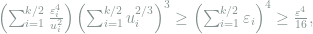
$\left(\sum_{i=1}^{k/2} \frac{\varepsilon_i^4}{u_i^2} \right) \left(\sum_{i=1}^{k/2} u_i^{2/3}\right)^3 \ge \left(\sum_{i=1}^{k/2} \varepsilon_i\right)^4 \ge \frac{\varepsilon^4}{16},$

which gives the lower bound $\sum_{i=1}^{k/2} \varepsilon_i^4/u_i^2 \ge \varepsilon^4/(16\|U\|_{2/3}^2)$ , with identity when

$\varepsilon_i = \varepsilon u_i^{2/3}/(2\|U\|_{2/3}^{2/3}).$

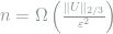
It is straightforward to check that $\varepsilon_i \le u_i$ for all $i$ thanks to the assumption $u_i\ge \varepsilon^3/8$ . Consequently, we arrive at the lower bound

$n = \Omega\left(\frac{\|U\|_{2/3}}{\varepsilon^2} \right)$

for the sample complexity, which is tight in general. Recall that how the mysterious $(2/3)$ -norm is obtained by carefully choosing the mixture.

3. Examples of Estimation Problems

In this section, we will look at several estimation problems and show how Theorem 1 provides the tight lower bound for these problems. We will see that the choice of the mixture becomes natural after we understand the problem.

3.1. Linear Functional Estimation of Sparse Gaussian Mean

Consider a Gaussian location model 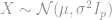$X\sim \mathcal{N}(\mu, \sigma^2I_p)$ , where we assume that the mean vector $\mu$ is $s$ -sparse, i.e., $\|\mu\|_0\le s$ . The target is to estimate the linear functional of $\mu$ , i.e., $L(\mu):= \sum_{i=1}^p \mu_i$ , and we aim to prove a tight minimax lower bound for the minimax risk $R_{s,p,\sigma}^\star$ under the quadratic loss.

The key feature of this problem is the dependence of the minimax risk on the sparsity parameter $s$ . If one could know the support of $\mu$ , summing over $X_i$ for $i\in \text{supp}(\mu)$ gives a natural estimator with risk $O(s\sigma^2)$ . However, due to the unknown support of $\mu$ , we will show that $R_{s,p,\sigma}^\star = \Omega(s^2\sigma^2\log p)$ for small $s$ , where the additional penalty $s\log p$ is essentially the logarithm of $\binom{p}{s}$ , the number of possible supports of $\mu$ .

To incorporate the effect of unknown support into the lower bound, a natural choice would be to consider a random mean vector with support uniformly distributed on all size- $s$ subsets of $[p]$ . Formally, let $P=\mathcal{N}(0,\sigma^2I_p)$ , and $Q_S = \mathcal{N}(\rho 1_S, \sigma^2 I_p)$ with $1_S$ being the indicator vector of the subset $S\subseteq [p]$ , and $\rho>0$ is a parameter to be specified. Moreover, we let $S$ be uniformly distributed on all possible size- $s$ subsets of $[p]$ . Clearly, the separability condition in Theorem 1 is satisfied with $\Delta = s^2\rho^2/2$ . To upper bound the $\chi^2$ -divergence, we again compute

$\int \frac{dQ_S dQ_{S'}}{dP} = \exp\left(\frac{\rho^2}{\sigma^2} |S\cap S'|\right),$

and consequently

$\chi^2\left(\mathop{\mathbb E}_S[Q_S], P \right) = \mathop{\mathbb E}_{S,S'} \exp\left(\frac{\rho^2}{\sigma^2} |S\cap S'|\right) - 1.$

The random variable $|S\cap S'|$ follows a hypergeometric distribution with pmf $\mathop{\mathbb P}(|S\cap S'| = r) = \binom{s}{r}\binom{p-s}{s-r} / \binom{p}{s}$ . It is well-known in probability theory that a hypergeometric distribution refers to sampling without replacement, while the Binomial distribution $\mathsf{B}(s,s/p)$ refers to sampling with replacement. The next lemma shows a relationship between these two random variables.

Lemma 4 Let $\{x_1,\cdots,x_M\}$ be an urn, $X_1,\cdots,X_n$ be samples uniformly drawn from the urn without replacement, and $X_1^\star, \cdots, X_n^\star$ be samples uniformly drawn from the urn with replacement. Define $S_n = \sum_{i=1}^n X_i$ and $S_n^\star = \sum_{i=1}^n X_i^\star$ , then there exists a coupling between $(S_n, S_n^\star)$ such that $\mathop{\mathbb E}[S_n^\star|S_n] = S_n$ .

Proof: The coupling is defined as follows: for any distinct $y_1,\cdots,y_n \in \{x_1,\cdots,x_M\}$ and not necessarily distinct $z_1,\cdots,z_n\in \{y_1,\cdots,y_n\}$ , let the conditional distribution be

$\mathop{\mathbb P}(X_1^\star = z_1, \cdots, X_n^\star = z_n | X_1 = y_1, \cdots, X_n = y_n) = \frac{\binom{M}{n}}{M^n\binom{M-L}{n-L}},$

where $L$ denotes the number of distinct elements in $z_1,\cdots,z_n$ . To verify that this is a valid conditional probability measure, recall that the number of ways of drawing $n$ labeled elements with $L$ distinct elements from an urn of $n$ elements is $S(n,L)(n)_L$ , where $S(n,L)$ is the Stirling’s number of the second kind, and $(n)_L := n! / (n-L)!$ is the falling factorial. Hence, the probability is valid due to the identity

$\sum_{L=1}^n \frac{\binom{M}{n}}{M^n\binom{M-L}{n-L}}\cdot S(n,L)(n)_L = \frac{1}{M^n}\sum_{L=1}^n S(n,L)(M)_L = 1,$

where the last step is due to that $\sum_{L=1}^n S(n,L)(M)_L$ is the number of ways of drawing $n$ labeled elements from an urn of $M$ elements and therefore equals $M^n$ .

From this conditional probability, it is obvious to see that the unconditional probability of $(X_1^\star, \cdots, X_n^\star)$ coincides with sampling with replacement. Moreover,

$\sum_{i=1}^n \mathop{\mathbb P}(X_i^\star = y| X_1 = y_1, \cdots, X_n = y_n) = 1(y\in \{y_1,\cdots,y_n\})$

follows from symmetry, and therefore $\mathop{\mathbb E}[S_n^\star|S_n] = S_n$ . $\Box$

By Lemma 4, there exists some $\sigma$ -algebra $\mathcal{B}$ such that $|S\cap S'|$ has the same distribution as $\mathop{\mathbb E}[Z|\mathcal{B}]$ with $Z\sim \mathsf{B}(s,s/p)$ . Now by Jensen’s inequality,

$\chi^2\left(\mathop{\mathbb E}_S[Q_S], P \right) \le \mathop{\mathbb E} \exp(\rho^2 Z/\sigma^2 ) - 1 = \left(1 - \frac{s}{p} + \frac{s}{p}\exp(\rho^2/\sigma^2) \right)^s - 1.$

Hence, the largest $\rho^2$ to ensure a constant $\chi^2$ -divergence is $\rho^2 = \sigma^2\log(1+p/s^2)$ , which by Theorem 1 gives

$R_{s,p,\sigma}^\star = \Omega\left(\sigma^2 s^2 \log\left(1+ \frac{p}{s^2}\right)\right),$

which has a phase transition at $s\sim \sqrt{p}$ . In fact, this lower bound is also tight: if $s \ge \sqrt{p}$ , the natural estimator $\sum_{i=1}^p X_i$ is rate-optimal; if $s<\sqrt{p}$ , the thresholding estimator $\sum_{i=1}^p X_i1(|X_i|\ge t)$ is rate-optimal for some proper threshold $t$ .

3.2. Largest Eigenvalue of Covariance Matrix

Consider i.i.d. observations $X_1,\cdots,X_n\sim \mathcal{N}(0,\Sigma)$ , where $\Sigma\in {\mathbb R}^{p\times p}$ is the covariance matrix. Assuming $\|\Sigma\|_{\text{op}}\le 1$ , classical matrix concentration inequality shows that the empirical covariance matrix $\hat{\Sigma} := n^{-1}\sum_{i=1}^n X_iX_i^\top$ satisfies that

$\mathop{\mathbb E}\|\hat{\Sigma} - \Sigma\|_{\text{op}} = O\left(\sqrt{\frac{p}{n}}\right).$

We show that the $\sqrt{p/n}$ bound is rate-optimal. In fact, we may even show a stronger result: the minimax risk $R_{n,p}^\star$ in estimating $\|\Sigma\|_{\text{op}}$ under the absolute value loss is at least

$R_{n,p}^\star = \Omega\left( 1 \wedge \sqrt{\frac{p}{n}}\right).$

Note that by triangle inequality, estimating the largest eigenvalue is indeed an easier problem than covariance estimation.

As before, a natural idea to establish the lower bound is to choose a uniform direction for the principal eigenvector, so that the learner must distribute her effort into all directions evenly. Specifically, we choose $P = \mathcal{N}(0, aI_p)$ , and $Q_v = \mathcal{N}(0,aI_p + bvv^\top)$ , where $a,b>0$ are some parameters to be chosen later, and $v$ is uniformly distributed on the unit ball $\{v\in {\mathbb R}^p: \|v\|_2 =1 \}$ . It is easy to verify that $\|\Sigma\|_{\text{op}}\le 1$ is fulfilled as long as $a+b\le 1$ , and $\Delta = b$ in Theorem 1. Moreover,

$\int \frac{dQ_vdQ_{v'}}{dP} = \left( 1 - \frac{b^2}{a^2}(v^\top v')^2 \right)^{-\frac{1}{2}}.$

Hence, by Lemma 2,

$\chi^2\left(\mathop{\mathbb E}_v[Q_v^{\otimes n}], P^{\otimes n}\right) +1 = \mathop{\mathbb E}_{v,v'} \left( 1 - \frac{b^2}{a^2}(v^\top v')^2 \right)^{-\frac{n}{2}} \le \mathop{\mathbb E}_{v,v'} \exp\left(\frac{nb^2}{a^2}(v^\top v')^2 \right)$

assuming $b/a\le 1/2$ , where the last inequality follows from $1-x \ge \exp(-2x)$ whenever $0\le x\le 1/4$ . Computation the surface area of spherical caps gives

$\mathop{\mathbb P}(|v^\top v'| \ge t) = \frac{1}{\text{Beta}(\frac{p-1}{2}, \frac{1}{2})}\int_0^{1-t^2} x^{\frac{p-3}{2}}(1-x)^{-\frac{1}{2}}dx = \exp(-\Omega(pt^2)).$

Consequently, to make $\chi^2\left(\mathop{\mathbb E}_v[Q_v^{\otimes n}], P^{\otimes n}\right) = O(1)$ , we may take

$a = \frac{1}{2}, \qquad b = \frac{1}{4} \wedge \sqrt{\frac{p}{n}},$

which gives the desired minimax lower bound $R_{n,p}^\star = \Omega\left( 1 \wedge \sqrt{p/n}\right)$ .

3.3. Quadratic Functional Estimation

Finally we switch to a non-parametric example. Let $X_1,\cdots,X_n$ be i.i.d. observations drawn from a density $f$ , where $f$ is supported on $[0,1]$ and belongs to the Hölder ball with smoothness parameter $s>0$ :

$f\in \mathcal{H}^s(L) := \left\{f\in C[0,1]: \sup_{x\neq y} \frac{|f^{(m)}(x) - f^{(m)}(y)| }{|x-y|^\alpha}\le L \right\},$

with $s = m+\alpha, m\in \mathbb{N}, \alpha\in (0,1]$ . The target is to estimate the quadratic functional

$Q(f) := \int_0^1 f(x)^2 dx,$

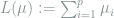
and we let $R_{n,s}^\star$ be the corresponding minimax risk under the absolute value loss. The central claim is that

$R_{n,s}^\star = \Omega\left( n^{-\frac{4s}{4s+1}} + n^{-\frac{1}{2}}\right),$

which has an “elbow effect” at $s=1/4$ .

A central tool for proving nonparametric lower bounds is via parametric reduction, i.e., restricting $f$ to a parametric family while the subproblem is as hard as the original nonparametric problem. In this example, a natural candidate is

$f_v(x) = 1 + c_0L\cdot \sum_{i=1}^{h^{-1}/2} v_ih^s\left[ g\left(\frac{x-(2i-2)h}{h} \right) - g\left(\frac{x-(2i-1)h}{h} \right) \right],$

where $h\in (0,1)$ is the bandwidth to be chosen later, the vector $v$ satisfies $\|v\|_\infty\le 1$ , and $g$ is a fixed smooth function on ${\mathbb R}$ vanishing outside $[0,1]$ . It is a simple exercise to show that for $c_0>0$ sufficiently small, each $f_v$ is a valid density on $[0,1]$ and belongs to the Hölder ball $\mathcal{H}^s(L)$ . Intuitively, the density $f_v$ is a perturbation on the uniform density with bumps modulated by the vector $v$ . Moreover,

$Q(f_v) = 1 + (c_0L\|g\|_2)^2 h^{2s+1} \cdot\|v\|_2^2,$

and therefore the target of the subproblem is to estimate $\|v\|_2^2$ based on $X_1,\cdots,X_n\sim f_v$ . Again, the idea of Theorem 1 can be applied.

Let $v$ be uniformly distributed on $\{\pm 1\}^{1/(2h)}$ . By simple calculation,

$\int_0^1 \frac{f_v(x)f_{v'}(x)}{f_0(x)}dx = 1 + (c_0L\|g\|_2)^2h^{2s+1}\cdot v^\top v'.$

Consequently, Lemma 2 gives

$\begin{array}{rcl} \chi^2\left(\mathop{\mathbb E}_v[f_v^{\otimes n}], f_0^{\otimes n} \right) + 1 &=& \mathop{\mathbb E}_{v,v'} \left(1 + (c_0L\|g\|_2)^2h^{2s+1}\cdot v^\top v' \right)^n \\ &\le & \mathop{\mathbb E}_{v,v'} \exp\left( (c_0L\|g\|_2)^2nh^{2s+1}\cdot v^\top v'\right) \\ &\le& \exp\left(\frac{1}{2}(c_0L\|g\|_2)^4n^2h^{4s+2}\cdot \frac{1}{2h} \right). \end{array}$

Hence, choosing $h = \Theta(n^{-\frac{2}{4s+1}})$ gives $\chi^2\left(\mathop{\mathbb E}_v[f_v^{\otimes n}], f_0^{\otimes n} \right) = O(1)$ . Moreover, Theorem 1 is fulfilled with $\Delta = \Theta(h^{2s}) = \Theta(n^{-\frac{4s}{4s+1}})$ , and therefore we have proved that

$R_{n,s}^\star = \Theta(n^{-\frac{4s}{4s+1}}).$

The parametric rate $R_{n,s}^\star = \Theta(n^{-1/2})$ is trivial (by the tools in Lecture 4).

4. Bibliographic Notes

A wonderful book which treats the point-mixture idea of Theorem 1 sysmatically and contains the method in Lemma 2 is Ingster and Suslina (2012). The sharp bounds on the clique size in the hidden clique problem are due to Matula (1972). It is a long-standing open problem whether there exists a polynomial-time algorithm attaining this statistical limit, and we refer to the lecture notes Lugosi (2017) for details. The sample complexity of the uniformity testing problem is due to Paninski (2008), and the general identity testing problem is studied in Valiant and Valiant (2017). There are also some other generalizations or tools for uniformity testing, e.g., Diakonikolas and Kane (2016), Diakonikolas, Kane and Stewart (2018), Blais, Canonne and Gur (2019).

For the estimation problem, the linear functional estimation for sparse Gaussian mean is due to Collier, Comminges and Tsybakov (2017), where Lemma 4 can be found in Aldous (1985). The largest eigenvalue example is taken from the lecture note Wu (2017). The nonparametric functional estimation problem is widely studied in statistics, where the minimax rate for estimating the quadratic functional can be found in Bickel and Ritov (1988), and it is $\Theta(n^{-\frac{4s}{4s+d}} + n^{-\frac{1}{2}})$ for general dimension $d$ . The same minimax rate (and the elbow effect) actually holds for all smooth functionals, see Birgé and Massart (1995), Kerkyacharian and Picard (1996) and Robins et al (2017).

Yuri Ingster and Irina A. Suslina. Nonparametric goodness-of-fit testing under Gaussian models. Vol. 169. Springer Science & Business Media, 2012.
David W. Matula. Employee party problem. Notices of the American Mathematical Society. Vol. 19, No. 2, 1972.
Gábor Lugosi. Lectures on Combinatorial Statistics. 2017.
Liam Paninski. A coincidence-based test for uniformity given very sparsely sampled discrete data. IEEE Transactions on Information Theory 54.10 (2008): 4750–4755.
Gregory Valiant and Paul Valiant. An automatic inequality prover and instance optimal identity testing. SIAM Journal on Computing 46.1 (2017): 429–455.
Ilias Diakonikolas and Daniel M. Kane. A new approach for testing properties of discrete distributions. 2016 IEEE 57th Annual Symposium on Foundations of Computer Science (FOCS). IEEE, 2016.
Ilias Diakonikolas, Daniel M. Kane, and Alistair Stewart. Sharp bounds for generalized uniformity testing. Advances in Neural Information Processing Systems. 2018.
Eric Blais, Clément L. Canonne, and Tom Gur. Distribution testing lower bounds via reductions from communication complexity. ACM Transactions on Computation Theory (TOCT) 11.2 (2019): 6.
Olivier Collier, Laëtitia Comminges, and Alexandre B. Tsybakov. Minimax estimation of linear and quadratic functionals on sparsity classes. The Annals of Statistics 45.3 (2017): 923–958.
David J. Aldous. Exchangeability and related topics. Ecole d’Eté de Probabilités de Saint-Flour XIII-1983. Springer, Berlin, Heidelberg, 1985. 1–198.
Yihong Wu. Lecture notes for ECE598YW: Information-theoretic methods for high-dimensional statistics. 2017.
Peter J. Bickel and Yaacov Ritov. Estimating integrated squared density derivatives: sharp best order of convergence estimates. Sankhya: The Indian Journal of Statistics, Series A (1988): 381–393.
Lucien Birgé and Pascal Massart. Estimation of integral functionals of a density. The Annals of Statistics 23.1 (1995): 11–29.
Gérard Kerkyacharian and Dominique Picard. Estimating nonquadratic functionals of a density using Haar wavelets. The Annals of Statistics 24.2 (1996): 485-507.
James Robins, Lingling Li, Rajarshi Mukherjee, Eric Tchetgen Tchetgen, and Aad van der Vaart. Higher order estimating equations for high-dimensional models. Annals of statistics 45, no. 5 (2017): 1951.

The Informaticists

A take on the science of information

Lecture 6: Generalized Two-Point Method: Point vs. Mixture

Like this:

Related

Leave a Reply Cancel reply

Share this:

Like this:

Related

Leave a Reply Cancel reply