(Warning: These materials may be subject to lots of typos and errors. We are grateful if you could spot errors and leave suggestions in the comments, or contact the author at yjhan@stanford.edu.) 

This lecture starts to talk about specific tools and ideas to prove information-theoretic lower bounds. We will temporarily restrict ourselves to statistical inference problems (which most lower bounds apply to), where the presence of randomness is a key feature in these problems. Since the observer cannot control the realizations of randomness, the information contained in the observations, albeit not necessarily in a discrete structure (e.g., those in Lecture 2), can still be limited. In this lecture and subsequent ones, we will introduce the reduction and hypothesis testingideas to prove lower bounds of statistical inference, and these ideas will also be applied to other problems. 

1. Basics of Statistical Decision Theory 

To introduce statistical inference problems, we first review some basics of statistical decision theory. Mathematically, let be a collection of probability triplets indexed by , and the observation is a random variable following distribution for an unknown parameter in the known parameter set . The specific structure of is typically called models or experiments, for the parameter can represent different model parameters or theories to explain the observation . A decision rule, or a (randomized) estimator is a transition kernel from to some action space . Let be a loss function, where represents the loss of using action when the true parameter is . A central quantity to measure the quality of a decision rule is the risk in the following definition. 

Definition 1 (Risk) Under the above notations, the risk of the decision rule under loss function and the true parameter is defined as

Intuitively, the risk characterizes the expected loss (over the randomness in both the observation and the decision rule) of the decision rule when the true parameter is . When is a point mass for some deterministic function , we will also call as an estimator and the risk in (1) becomes 

Example 1 In linear regression model with random design, let the observations be i.i.d. with and . Here the parameter set is a finite-dimensional Euclidean space, and therefore we call this model parametric. The quantity of interest is , and the loss function may be chosen to be the prediction error of the linear estimator . 

Example 2 In density estimation model, let be i.i.d. drawn from some -Lipschitz density supported on . Here the parameter set of the unknown is the infinite-dimensional space of all possible -Lipschitz functions on , and we call this model non-parametric. The target may be to estimate the density at a point, the entire density, or some functional of the density. In respective settings, the loss functions can be

Example 3 By allowing general action spaces and loss functions, the decision-theoretic framework can also incorporate some non-statistical examples. For instance, in stochastic optimization may parameterize a class of convex Lipschitz functions , and denotes the noisy observations of the gradients at the queried points. Then the action space may just be the entire domain , and the loss function is the optimality gap defined as

In practice, one would like to find optimal decision rules for a given task. However, the risk is a function of and it is hard to compare two risk functions directly. Hence, people typically map the risk functions into scalars and arrive at the following minimax and Bayesian paradigm. 

Definition 2 (Minimax and Bayes Decision Rule) The minimax decision rule is the decision rule which minimizes the quantity . The Bayes decision rule under distribution (called the prior distribution) is the decision rule which minimizes the quantity . 

It is typically hard to find the minimax decision rule in practice, while the Bayes decision rule admits a closed-form expression (although hard to compute in general). 

Proposition 3 The Bayes decision rule under prior is given by the estimator

where denotes the posterior distribution of under (assuming the existence of regular posterior). 

Proof: Left as an exercise for the reader.  

2. Deficiency and Model Distance 

The central target of statistical inference is to propose some decision rule for a given statistical model with small risks. Similarly, the counterpart in the lower bound is to prove that certain risks are unavoidable for any decision rules. Here to compare risks, we may either compare the entire risk function, or its minimax or Bayes version. In this lecture we will focus on the risk function, and many later lectures will be devoted to appropriate minimax risks. 

We start with the task of comparing two statistical models with the same parameter set . Intuitively, one may think that the model with a smaller noise level would be better than the other, e.g., the model should be better than . However, this criterion is bad due to two reasons: 

1. There is no proper notion of noise for general (especially non-additive) statistical models; 
2. Even if a natural notion of noise exists for certain models, it is not necessarily true that the model with smaller noise is always better. For example, let
   the model has a smaller magnitude of the additive noise. However, despite with a larger magnitude of the noise, the model is actually noise-free since one can decode the perfect knowledge of from the observation. 

To overcome the above difficulties, we introduce the idea of model reduction. Specifically, we aim to establish the fact that for any decision rule in one model, there is another decision rule in the other model which is uniformly no worse than the former rule. The idea of reduction appears in many fields, e.g., in P/NP theory it is sufficient to work out one NP-complete instance (e.g., circuit satisfiability) from scratch and establish all others by polynomial reduction. This reduction idea is made precise via the following definition. 

Definition 4 (Model Deficiency) For two statistical models and , we call is -deficient relative to if for any finite subset , any finite action space , any loss function , and any decision rule based on model , there exists some decision rule based on model such that

Note that the definition of model deficiency does not involve the specific choice of the action space and loss function, and the finiteness of and in the definition is mainly for technical purposes. Intuitively speaking, is -deficient relative to if the entire risk function of some decision rule in is no worse than that of any given decision rule in , within an additive gap . 

Although Definition 4 gives strong performance guarantees for the -deficient model , it is difficult to verify the condition (4), i.e., to transform an arbitrary decision rule to some proper . A crucial observation here is that it may be easier to transform between models and , and in particular, when is a randomization of . For example, if there exists some stochastic kernel such that for all (where denotes the marginal distribution of the output of kernel with input distributed as ), then we may simply set to arrive at (4) with . The following theorem shows that model deficiency is in fact equivalent to approximate randomization. 

Theorem 5 Model is -deficient with respect to if and only if there exists some stochastic kernel such that

where is the total variation distance between probability measures and . 

Proof: The sufficiency part is easy. Given such a kernel and a decision rule based on model , we simply set , i.e., transmit the output through kernel and apply . Then for any , 

for the loss function is non-negative and upper bounded by one. 

The necessity part is slightly more complicated, and for simplicity we assume that all are finite (the general case requires proper limiting arguments). In this case, any decision rules or , loss functions and priors can be represented by a finite-dimensional vector. Given and , the condition (4) ensures that 

Note that the LHS of (5) is bilinear in and , both of which range over some convex sets (e.g., the domain for is exactly ), the minimax theorem allows to swap and of (5) to obtain that 

By evaluating the inner supremum, (6) implies the existence of some such that 

Finally, choosing and in (7), the corresponding is the desired kernel .  

Based on the notion of deficiency, we are ready to define the distance between statistical models, also known as the Le Cam’s distance. 

Definition 6 (Le Cam’s Distance) For two statistical models and with the same parameter set , Le Cam’s distance is defined as the infimum of such that is -deficient relative to , and is -deficient relative to . 

It is a simple exercise to show that Le Cam’s distance is a pesudo-metric in the sense that it is symmetric and satisfies the triangle inequality. The main importance of Le Cam’s distance is that it helps to establish equivalence between some statistical models, and people are typically interested in the case where or . The main idea is to use randomization (i.e., Theorem 5) to obtain an upper bound on Le Cam’s distance, and then apply Definition 4 to deduce useful results (e.g., to carry over an asymptotically optimal procedure in one model to other models). 

In the remainder of this lecture, I will give some examples of models whose distance is zero or asymptotically zero. In the next lecture it will be shown that regular models will always be close to some Gaussian location model asymptotically, and thereby the classical asymptotic theory of statistics can be established. 

3. Equivalence between Models 

3.1. Sufficiency 

We first examine the case where . By Theorem 5, models and are mutual randomizations. In the special case where is a deterministic function of (thus is the push-forward measure of through ), we have the following result. 

Theorem 7 Under the above setting, if and only if forms a Markov chain. 

Note that the Markov condition is the usual definition of sufficient statistics, and also gives the well-known Rao–Blackwell factorization criterion for sufficiency. Hence, sufficiency is in fact a special case of model equivalence, and deficiency can be thought of as approximate sufficiency. 

3.2. Equivalence between Multinomial and Poissonized Models 

Consider a discrete probability vector with . A widely-used model in practice is the multinomial model , which models the i.i.d. sampling process and draws i.i.d. observations . However, a potential difficulty in handling multinomial models is that the empirical frequencies of symbols are dependent, which makes the analysis annoying. To overcome this difficulty, a common procedure is to consider a Poissonized model , where we draw a Poisson random variable first and observes i.i.d. . Due to the nice properties of Poisson random variables, the empirical frequencies now follow independent scaled Poisson distribution. 

The next theorem shows that the multinomial and Poissonized models are asymptotically equivalent, which means that it actually does no harm to consider the more convenient Poissonized model for analysis, at least asymptotically. In later lectures I will also show a non-asymptotic result between these two models. 

Theorem 8 For fixed , . 

Proof: We only show that is -deficient relative to , with , where the other direction is analogous. By Theorem 5, it suffices to show that is an approximate randomization of . The randomization procedure is as follows: based on the observations under the multinomial model, let be the vector of empirical frequencies. Next draw an independent random variable . If , let be the output of the kernel. Otherwise, we generate i.i.d. samples , and let be the output. We remark that it is important that the above randomization procedure does not depend on the unknown . 

Let be the distribution of the Poissonized and randomized model under true parameter , respectively. Now it is easily shown that 

where , denotes the -fold produce of , takes the expectation w.r.t. , and takes the expectation w.r.t. random samples . To upper bound the total variation distance in (8), we shall need the following lemma. 

Lemma 9 Let and be the KL divergence and -divergence, respectively. Then

The proof of Lemma 9 will be given in later lectures when we talk about joint ranges of divergences. Then by Lemma 9 and Jensen’s inequality, 

Since by simple algebra, 

then by (8) we obtain that 

which goes to zero uniformly in as , as desired.  

Remark 1 In fact, the following non-asymptotic characterization

could be established. This result is contained in an upcoming paper.

3.3. Equivalence between Nonparametric Regression and Gaussian White Noise Models 

A well-known problem in nonparametric statistics is the nonparametric regression: 

where the underlying regression function is unknown, and is some noise level. Typically, the statistical goal is to recover the function at some point or globally, and some smoothness conditions are necessary to perform this task. A typical assumption is that belongs to some H\”{o}lder ball, where 

with denotes the smoothness parameter. 

There is also a continuous version of (9) called the Gaussian white noise model, where a process satisfying the following stochastic differential equation is observed: 

where is the standard Brownion motion. Compared with the regression model in (9), the white noise model in (10) gets rid of the quantization issue of and is therefore easier to analyze. Note that in both models is effectively the sample size. 

Let be the regression and white noise models with known parameters and the paramter set , respectively. The main result in this section is that, when , these models are asymptotically equivalent. 

Theorem 10 If , we have . 

Proof: Consider another Gaussian white noise model where the only difference is to replace in (10) by defined as 

Note that under the same parameter , we have 

which goes to zero uniformly in as . Therefore, by Theorem 5 and Lemma 9, we have . On the other hand, in the model the likelihood ratio between the signal distribution and the pure noise distribution is 

As a result, under model , there is a Markov chain . Since under the same parameter , under is identically distributed as under , by Theorem 7 we have exact sufficiency and conclude that . Then the rest follows from the triangle inequality.  

3.4. Equivalence between Density Estimation and Gaussian White Noise Models 

Another widely-used model in nonparametric statistics is the density estimation model, where samples are i.i.d. drawn from some unknown density . Typically some smoothness condition is also necessary for the density, and we assume that again belongs to the H\”{o}lder ball. 

Compared with the previous results, a slightly more involved result is that the density estimation model, albeit with a seemingly different form, is also asymptotically equivalent to a proper Gaussian white noise model. However, here the Gaussian white noise model should take the following different form: 

In other words, in nonparametric statistics the problems of density estimation, regression and estimation in Gaussian white noise are all asymptotically equivalent, under certtain smoothness conditions. 

Let be the density estimation model and the Gaussian white noise model in (11), respectively. The main result is summarized in the following theorem. 

Theorem 11 If and the density is bounded below from zero everywhere, then . 

Proof: Instead of the original density estimation model, we actually consider a Poissonized sampling model instead, where the observation under is a Poisson process on with intensity . Similar to the proof of Theorem 8, we have and it remains to show that . 

Fix an equal-spaced grid in with , where is a small constant depending only on . Next we come up with two new models and , where the only difference is that the parameter is replaced by defined as 

As long as , the same arguments in the proof of Theorem 10 can be applied to arrive at (for the white noise model, the assumption that is bounded away from zero ensures the smoothness of ). Hence, it further suffices to focus on the new models and show that . An interesting observation is that under the model , the vector with 

is sufficient. Moreover, under the model , the vector with 

is also sufficient. Further, all entries of and are mutually independent. Hence, the ultimate goal is to find mutual randomizations between and for . 

To do so, a first attempt would be to find a bijective mapping independently for each . However, this approach would lose useful information from the neighbors as we know that thanks to the smoothness of . For example, we have with , and with . Motivated by this fact, we represent and in the following bijective way (assume that is even): 

Note that is again an independent Poisson vector, we may repeat the above transformation for this new vector. Similar things also hold for . Hence, at each iteration we may leave half of the components unchanged, and apply the above transformations to the other half. We repeat the iteration for times (assuming is a power of ), so that finally we arrive at a vector of length consisting of sums. Let (resp. ) be the final vector of sums, and (resp. ) be the vector of remaining entries which are left unchanged at some iteration. 

Remark 2 Experienced readers may have noticed that these are the wavelet coefficients under the Haar wavelet basis, where superscripts and stand for father and mother wavelets, respectively. 

Next we are ready to describe the randomization procedure. For notational simplicity we will write as a representative example of an entry in , and write as a representative example of an entry in . 

For entries in , note that by the delta method, for , the random variable is approximately distributed as (in fact, the squared root is the variance-stabilizing transformation for Poisson random variables). The exact transformation is then given by 

where is an independent auxiliary variable. The mapping (12) is one-to-one and can thus be inverted as well. 

For entries in , we aim to use quantile transformations to convert to . For , let be the CDF of , and be the CDF of . Then the one-to-one quantile transformation is given by 

where again is an independent auxiliary variable. The output given by (13) will be expected to be close in distribution to , and the overall transformation is also invertible. 

The approximation properties of these transformations are summarized in the following theorem. 

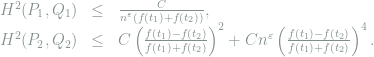
Theorem 12 Sticking to the specific examples of and , let be the respective distributions of the RHS in (12) and (13), and be the respective distributions of and , we have

where is some universal constant, and denotes the Hellinger distance. 

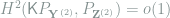
The proof of Theorem 12 is purely probabilitistic and involved, and is omitted here. Applying Theorem 12 to the vector of length , each component is the sum of elements bounded away from zero. Consequently, let be the overall transition kernel of the randomization, the inequality gives 

As for the vector , the components lie in possible different levels. At level , the spacing of the grid becomes , and there are elements. Also, we have at -th level, with . Consequently, 

Since , we may choose to be sufficiently small (i.e., ) to make . The proof is completed.  

4. Bibliographic Notes 

The statistical decision theory framework dates back to Wald (1950), and is currently the elementary course for graduate students in statistics. There are many excellent textbooks on this topic, e.g., Lehmann and Casella (2006) and Lehmann and Romano (2006). The concept of model deficiency is due to Le Cam (1964), where the randomization criterion (Theorem 5) was proved. The present form is taken from Torgersen (1991). We also refer to the excellent monographs by Le Cam (1986) and Le Cam and Yang (1990). 

The asymptotic equivalence between nonparametric models has been studied by a series of papers since 1990s. The equivalence between nonparametric regression and Gaussian white noise models (Theorem 10) was established in Brown and Low (1996), where both the fixed and random designs were studied. It was also shown in a follow-up work (Brown and Zhang 1998) that these models are non-equivalent if . The equivalence of the density estimation model and others (Theorem 11) was established in Brown et al. (2004), and we also refer to a recent work (Ray and Schmidt-Hieber 2016) which relaxed the crucial assumption that the density is bounded below from zero. Poisson approximation or Poissonization is a well-known technique widely used in probability theory, statistics and theoretical computer science, and the current treatment is essentially taken from Brown et al. (2004). 

1. Abraham Wald, Statistical decision functions. Wiley, 1950. 
2. Erich L. Lehmann and George Casella, Theory of point estimation. Springer Science & Business Media, 2006. 
3. Erich L. Lehmann and Joseph P. Romano, Testing statistical hypotheses. Springer Science & Business Media, 2006. 
4. Lucien M. Le Cam, Sufficiency and approximate sufficiency. The Annals of Mathematical Statistics (1964): 1419-1455. 
5. Erik Torgersen, Comparison of statistical experiments. Cambridge University Press, 1991. 
6. Lucien M. Le Cam, Asymptotic methods in statistical theory. Springer, New York, 1986. 
7. Lucien M. Le Cam and Grace Yang, Asymptotics in statistics. Springer, New York, 1990. 
8. Lawrence D. Brown and Mark G. Low, Asymptotic equivalence of nonparametric regression and white noise. The Annals of Statistics 24.6 (1996): 2384-2398. 
9. Lawrence D. Brown and Cun-Hui Zhang, Asymptotic nonequivalence of nonparametric experiments when the smoothness index is . The Annals of Statistics 26.1 (1998): 279-287. 
10. Lawrence D. Brown, Andrew V. Carter, Mark G. Low, and Cun-Hui Zhang, Equivalence theory for density estimation, Poisson processes and Gaussian white noise with drift. The Annals of Statistics 32.5 (2004): 2074-2097. 
11. Kolyan Ray, and Johannes Schmidt-Hieber, The Le Cam distance between density estimation, Poisson processes and Gaussian white noise. arXiv preprint arXiv:1608.01824 (2016).